1.1 Overview
What is the general workflow, steps, tools used and best practices for bulk rna-seq analysis?
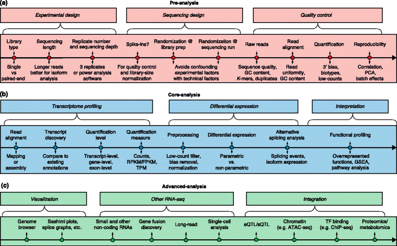
The major analysis steps are listed above the lines for pre-analysis, core analysis and advanced analysis. The key analysis issues for each step that are listed below the lines are discussed in the text. a Preprocessing includes experimental design, sequencing design, and quality control steps. b Core analyses include transcriptome profiling, differential gene expression, and functional profiling. c Advanced analysis includes visualization, other RNA-seq technologies, and data integration. Abbreviations: ChIP-seq Chromatin immunoprecipitation sequencing, eQTL Expression quantitative loci, FPKM Fragments per kilobase of exon model per million mapped reads, GSEA Gene set enrichment analysis, PCA Principal component analysis, RPKM Reads per kilobase of exon model per million reads, sQTL Splicing quantitative trait loci, TF Transcription factor, TPM Transcripts per million.
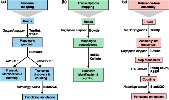
Three basic strategies for regular RNA-seq analysis. a An annotated genome is available and reads are mapped to the genome with a gapped mapper. Next (novel) transcript discovery and quantification can proceed with or without an annotation file. Novel transcripts are then functionally annotated. b If no novel transcript discovery is needed, reads can be mapped to the reference transcriptome using an ungapped aligner. Transcript identification and quantification can occur simultaneously. c When no genome is available, reads need to be assembled first into contigs or transcripts. For quantification, reads are mapped back to the novel reference transcriptome and further analysis proceeds as in (b) followed by the functional annotation of the novel transcripts as in (a). Representative software that can be used at each analysis step are indicated in bold text. Abbreviations: GFF General Feature Format, GTF gene transfer format, RSEM RNA-Seq by Expectation Maximization.
1.2 Experimental design
Are technical replicates needed for RNA-Seq analyses?
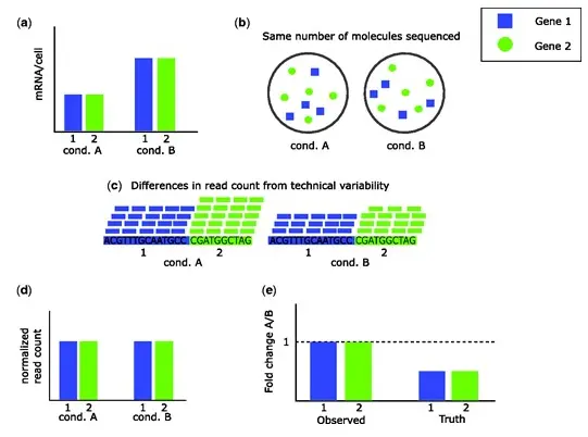
We find that the Illumina sequencing data are highly replicable, with relatively little technical variation, and thus, for many purposes, it may suffice to sequence each mRNA sample only once.
Marioni et al. (2008)
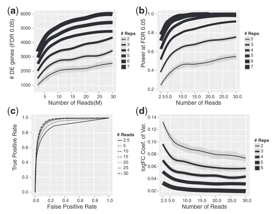
How many biological replicates are needed in an RNA-seq experiment?
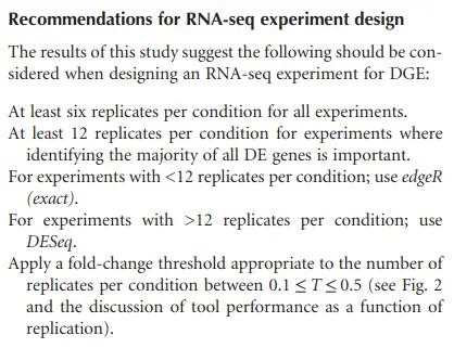
Schurch et al. (2016)
Number of replicates can be calculated more precisely using power analysis. RnaSeqSampleSize is an R package for power analysis and sample size estimation for RNA-Seq experiment.
Zhao et al. (2018)
RNASeqPower based spreadsheet (Google Sheet) and Shiny App.
Hart et al. (2013)
More sequencing depth or more biological replicates?
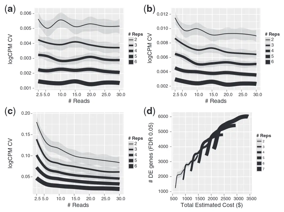
Y. Liu et al. (2014)
1.3 RNA extraction
Impact of RNA degradation on transcript quantification
We observed widespread effects of RNA quality on measurements of gene expression levels, as well as a slight but significant loss of library complexity in more degraded samples.
While standard normalizations failed to account for the effects of degradation, we found that by explicitly controlling for the effects of RIN using a linear model framework we can correct for the majority of these effects. We conclude that in instances in which RIN and the effect of interest are not associated, this approach can help recover biologically meaningful signals in data from degraded RNA samples.
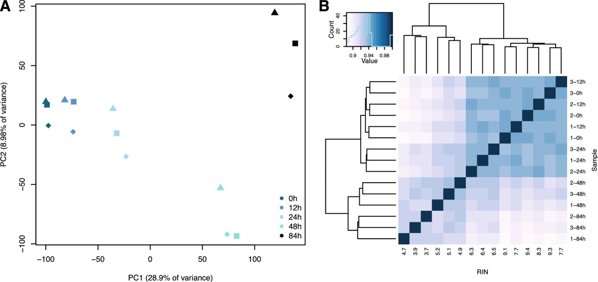
Gallego Romero et al. (2014)
Our current analyses indicate that structured small RNAs with low GC content are recovered inefficiently when a small number of cells is used for RNA isolation with TRIzol. We further find that, in addition to miRNAs, some pre-miRNAs, small interfering RNA (siRNA) duplexes, and transfer RNAs (tRNAs) are also extracted inefficiently under these conditions, reducing their representation in the pool of recovered RNAs.
Kim et al. (2012)
1.4 Library prep
As many as 1751 genes in Gencode Release 19 were identified to be differentially expressed when comparing stranded and non-stranded RNA-seq whole blood samples. Antisense and pseudogenes were significantly enriched in differential expression analyses. Because stranded RNA-seq retains strand information of a read, we can resolve read ambiguity in overlapping genes transcribed from opposite strands, which provides a more accurate quantification of gene expression levels compared with traditional non-stranded RNA-seq.
Stranded RNA-seq provides a more accurate estimate of transcript expression compared with non-stranded RNA-seq, and is therefore the recommended RNA-seq approach for future mRNA-seq studies.
1.5 Sequencing
Chhangawala et al. (2015), Corley et al. (2017), Y. Liu et al. (2014)
1.6 De novo assembly
1.7 PCR and deduplication
Fu et al. (2018), Parekh et al. (2016), Klepikova et al. (2017)
1.8 Mapping
Baruzzo et al. (2017)
1.9 Normalisation
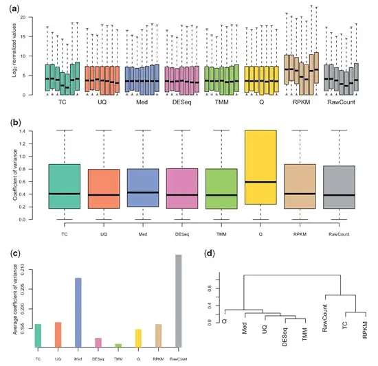
Dillies et al. (2013)
Evans et al. (2018)
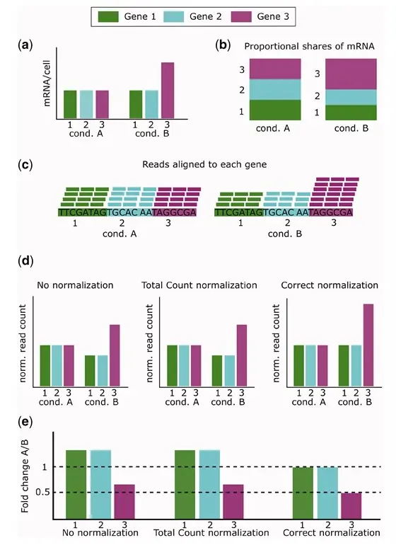
1.9.1 Use of RPKM & TPM
Issues with RPKM and suggestion for use of TPM.
Wagner et al. (2012)
Below is a suggested workflow to follow in order to compare RPKM or TPM values across samples. 1. Make sure both samples are sequenced using the same protocol in terms of strandedness. If not, samples cannot be compared. 2. Make sure both samples use the same RNA isolation approach (polyA+ selection vs ribosomal RNA depletion). If not, they should not be compared. 3. Check the fraction of the ribosomal, mitochondrial and globin RNAs, and the top highly expressed transcripts and see whether such RNAs constitute a very large part of the sequenced reads in a sample, and thus decrease the sequencing ‘real estate’ available for the remaining genes in that sample. If the calculated fractions in two samples differ significantly, do not compare RPKM or TPM values directly. TPM should never be used for quantitative comparisons across samples when the total RNA contents and its distributions are very different. However, under appropriate circumstances, TPM can be still useful for qualitative comparison such as PCA and clustering analysis.
Zhao et al. (2020)
1.10 Batch effect
1.11 Differential gene expression
Which DE tool should you use?
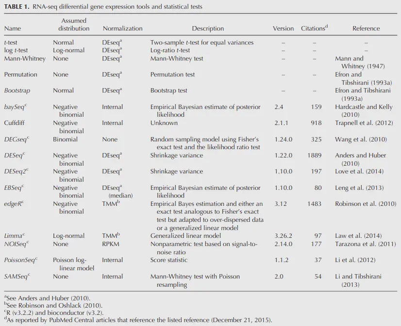
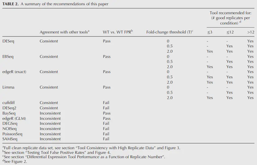
Schurch et al. (2016), Seyednasrollah et al. (2015)
1.11.1 Modelling in R
If variable is a factor, then the two models with and without the intercept term are equivalent, but if variable is a covariate (continuous) the then two models are fundamentally different.
In general, we suggest the inclusion of an intercept term for modelling explanatory variables that are covariates (continuous) since it provides a more flexible fit to the data points.
1.12 Celltype deconvolution
Nine methods were used to deconvolve celltypes from bulk PBMC RNA-seq data and simulated bulk data using single cell RNA-seq as reference.
Recommendations on reference data:
- Balanced sampling of single-cell data improves accuracy
- Enlarging reference datasets does not necessarily enhance accuracy and may introduce noise if expression patterns are already well captured
- Mismatch in cell types between reference and bulk samples significantly reduces accuracy. Best performance occurs when reference and bulk cell types are fully aligned
- Adding extra, irrelevant cell types to the reference can introduce confusion and worsen deconvolution performance
Performance insights:
- SVR-based methods outperform OLS-based methods overall
- AutoGeneS and CPM show strong predictive performance; AutoGeneS is also runtime-efficient
- DWLS performs best among OLS-based approaches and is particularly effective when gene expression collinearity is high
- ADAPTS (DCQ algorithm) and CPM are most robust when reference and bulk cell types are inconsistent
- Cell type subdivision improves performance for some tools (notably DWLS), highlighting sensitivity to gene co-expression structures
Xu et al. (2025)
1.13 Other
A benchmark for quantification pipelines
Teng et al. (2016)
1.14 Reference & File formats
- Illumina read quality scores
- Illumina read name format
- GTF format
- SAM file format
1.15 Software
1.15.1 Reads and general QC
1.15.2 Aligners (Mapper)
1.15.3 Pseudoaligners
1.15.4 Aligned QC
Tools to assess post-alignment quality, ie; after mapping of reads to a reference.
1.15.5 Quantification
1.15.6 Pipelines
1.15.6.1 Nextflow nf-core rnaseq
- Bulk RNA-Seq, SMART-Seq
- QC, trimming, UMI demultiplexing, mapping, quantification
- cellxgene matrix
- nf-core rnaseq
1.15.7 Genome browsers
Interactive exploration of BAM files, ie; reads aligned to a reference.
1.15.8 Batch correction
1.15.9 GSA/GSEA
- Convert gene IDs gProfiler
- OSA/ORA Online Enrichr
- OSA/ORA Online GOrilla
- OSA/ORA Online Panther
- ORA/GSEA/NTA Online Webgestalt
- ORA/GSEA Online DAVID
- KEGG pathways KEGG
- Functional annotation through orthology eggNOGmapper
- ORA/GSEA in R clusterProfiler
- Standalone software ErmineJ
- Plot genes on Kegg pathways in R Pathview
- Cytoscape plugin ClueGO
- Semantic reduction of terms ReviGO
1.15.10 GUI
Graphical User Interfaces for analysis of RNA-Seq data.
1.16 Courses, Workshops & Tutorials
- University of Cambridge workshop
- Bioconductor RNA-Seq workflow in R rnaseqGene
- Griffith Lab RNA-Seq tutorial
1.17 Other
Estimating storage requirements for FASTQ files
- One .fastq file for Single-End sequencing
- .fastq MB = Number of million reads x (60 + 2 x read length in bp)
- Paired-End sequencing produces 2 fastq files
- .fastq MB = Number of million reads x (60 + 2 x read length in bp) x 2
- It is recommended to store .fastq files in a compressed format (ex: .gz), which makes the file approximately 4 times smaller.
Elixir (2022)