---
title: ObservableJS in Quarto
subtitle: "Recreating ggplot plots using OJS"
author: "Roy Francis"
date: last-modified
date-format: "DD-MMM-YYYY"
format:
html:
page-layout: full
fig-align: left
title-block-banner: true
code-tools: true
code-overflow: wrap
toc: true
execute:
echo: true
---
This is recreated from [here](https://rud.is/wpe-plot/).
```{r}
#| filename: R
library(ggplot2)
head(mtcars)
```
## Read data
Convert R object to OJS object.
```{r}
#| filename: R
ojs_define(ojs_mtcars = mtcars)
```
Transpose JS object. Preview of JSON object.
```{ojs}
//| filename: OJS
mtcars = transpose(ojs_mtcars)
mtcars
```
## Table
```{ojs}
viewof tbl_mtcars = Inputs.table(mtcars)
```
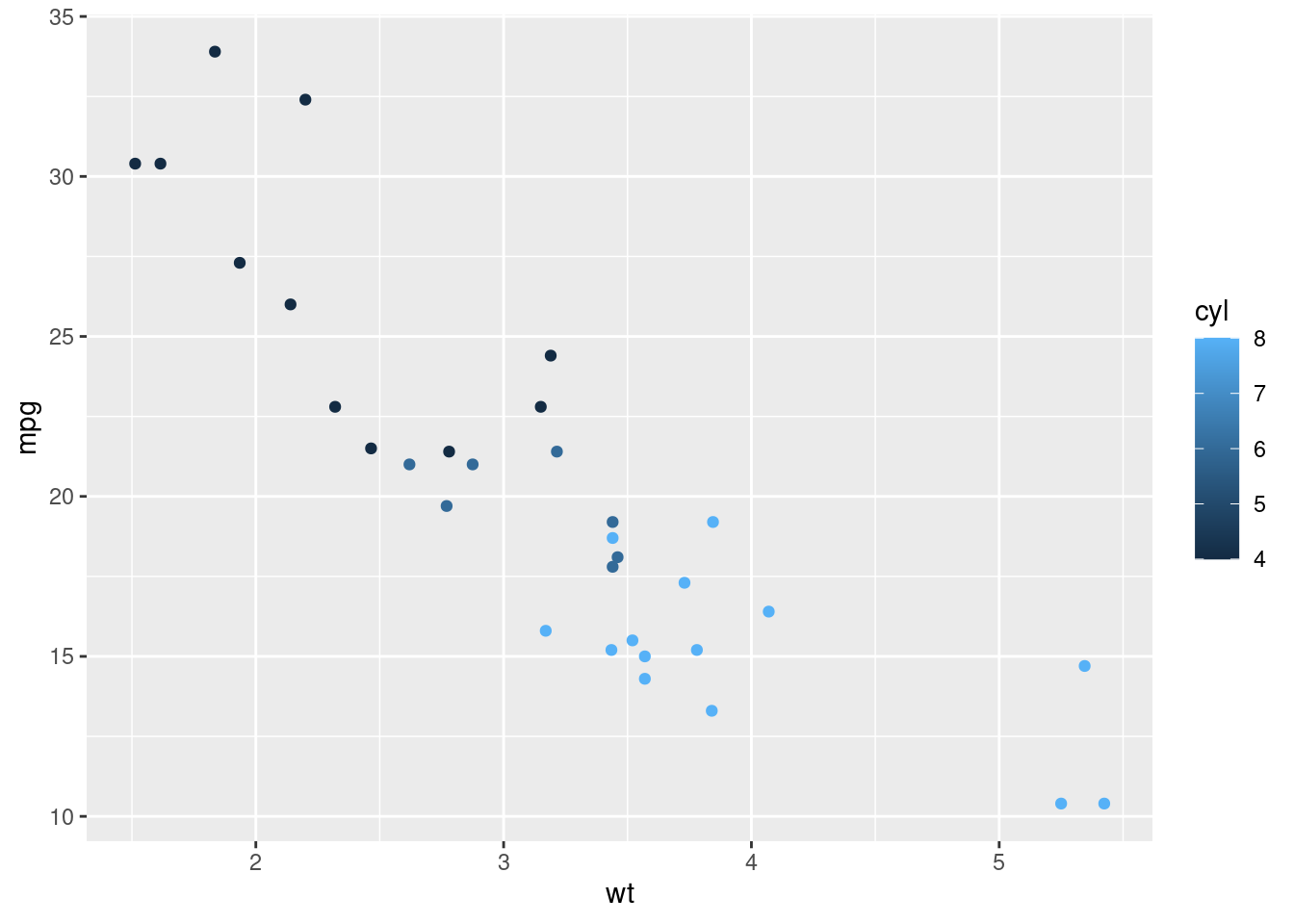
## Scatterplot
::: {.grid}
::: {.g-col-6}
```{r}
#| filename: R
ggplot(mtcars, aes(wt, mpg, col = cyl)) +
  geom_point()
```
:::
::: {.g-col-6}
```{ojs}
//| filename: OJS
plot_data = Plot.plot({
  color: { legend: true},
  marks: [
    Plot.dot(mtcars, {
      x: "wt",
      y: "mpg",
      fill: "cyl",
      tip: true,
      channels: { Name: "_row" }
    })
  ],
  grid: true
})
```
:::
:::
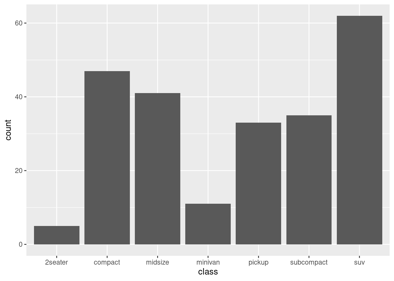
## Barplot
::: {.grid}
::: {.g-col-6}
```{r}
#| filename: R
ggplot(mpg, aes(class)) +
  geom_bar()
```
:::
::: {.g-col-6}
```{r}
#| filename: R
ojs_define(ojs_mpg = mpg)
```
```{ojs}
//| filename: OJS
mpg = transpose(ojs_mpg)
```
```{ojs}
//| filename: OJS
Plot.plot({
  marks: [
    Plot.auto(mpg, { x: "class", y: { reduce: "count" }, mark: "bar" })
  ],
  y: {
    grid: true,
  }
})
```
:::
:::
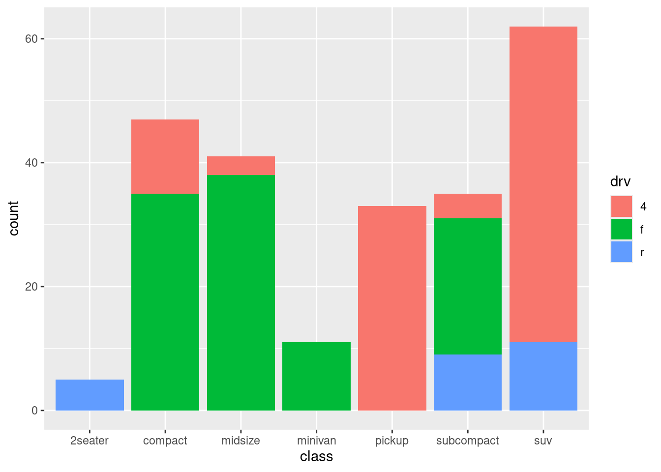
### With categorical colors
::: {.grid}
::: {.g-col-6}
```{r}
#| filename: R
ggplot(mpg, aes(class)) +
  geom_bar(aes(fill = drv))
```
:::
::: {.g-col-6}
```{ojs}
//| filename: OJS
Plot.plot({
  color: {
    legend: true
  },
  y: {
    grid: true,
  },
  marks: [
    Plot.auto(mpg, { x: "class", y: { reduce: "count" }, color: "drv", mark: "bar" })
  ]
})
```
:::
:::
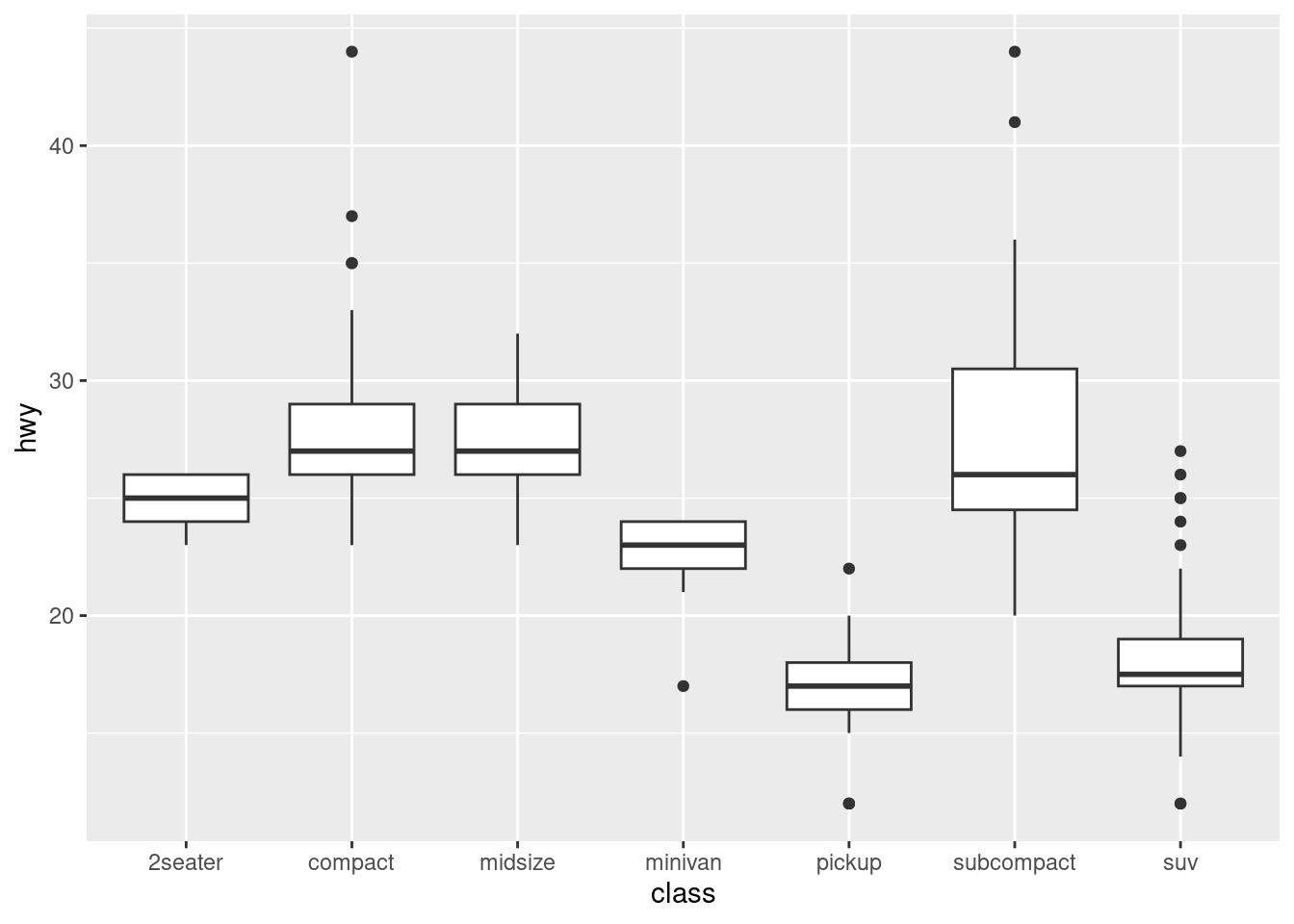
## Boxplot
::: {.grid}
::: {.g-col-6}
```{r}
#| filename: R
ggplot(mpg, aes(class, hwy)) +
  geom_boxplot()
```
:::
::: {.g-col-6}
```{ojs}
//| filename: OJS
Plot.plot({
  marks: [
    Plot.boxY(
      mpg,
      { x: "class", y: "hwy" }
    )
  ]
})
```
:::
:::
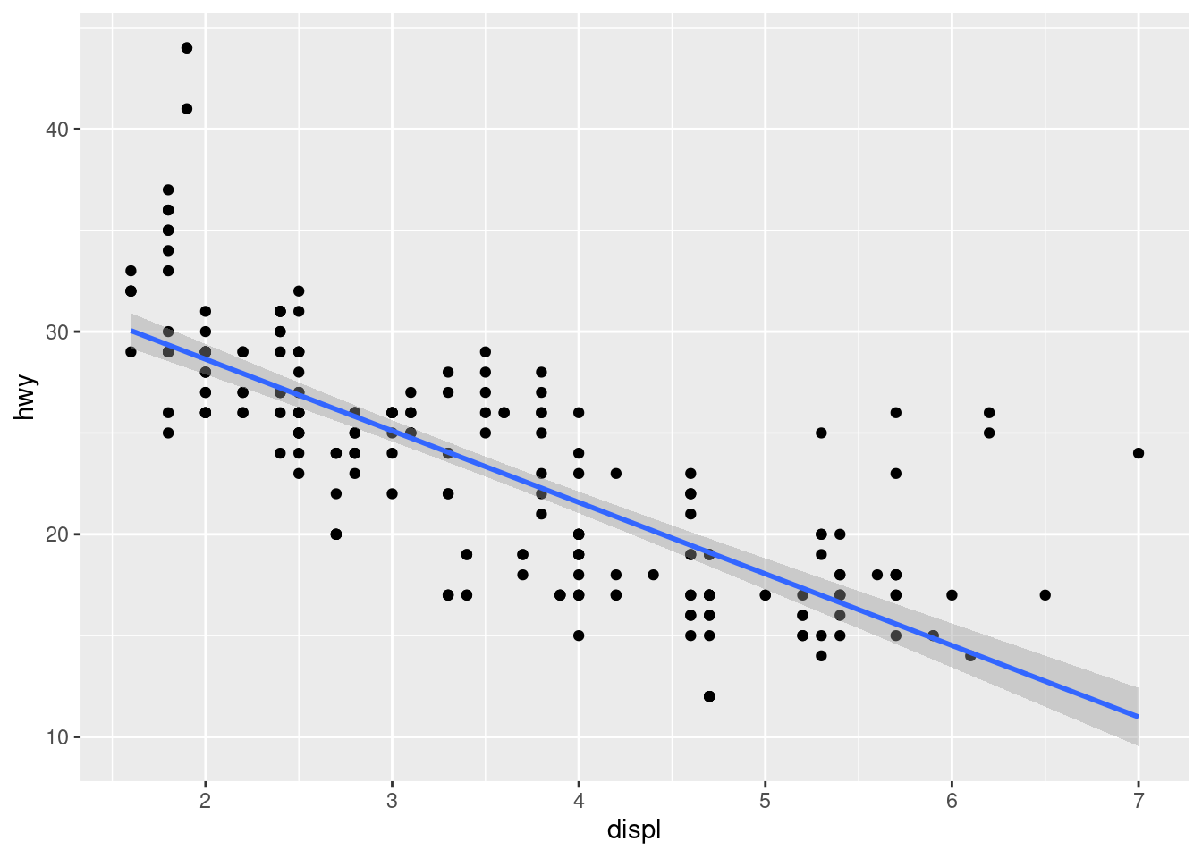
## Regression
::: {.grid}
::: {.g-col-6}
```{r}
#| filename: R
ggplot(mpg, aes(displ, hwy)) +
  geom_point() +
  geom_smooth(method="lm")
```
:::
::: {.g-col-6}
```{ojs}
//| filename: OJS
Plot.plot({
  marks: [
    Plot.dot(
      mpg,
      { x: "displ", y: "hwy" }
    ),
    Plot.linearRegressionY(
      mpg, {
      x: "displ",
      y: "hwy",
      stroke: "red",
    }),
  ],
})
```
:::
:::
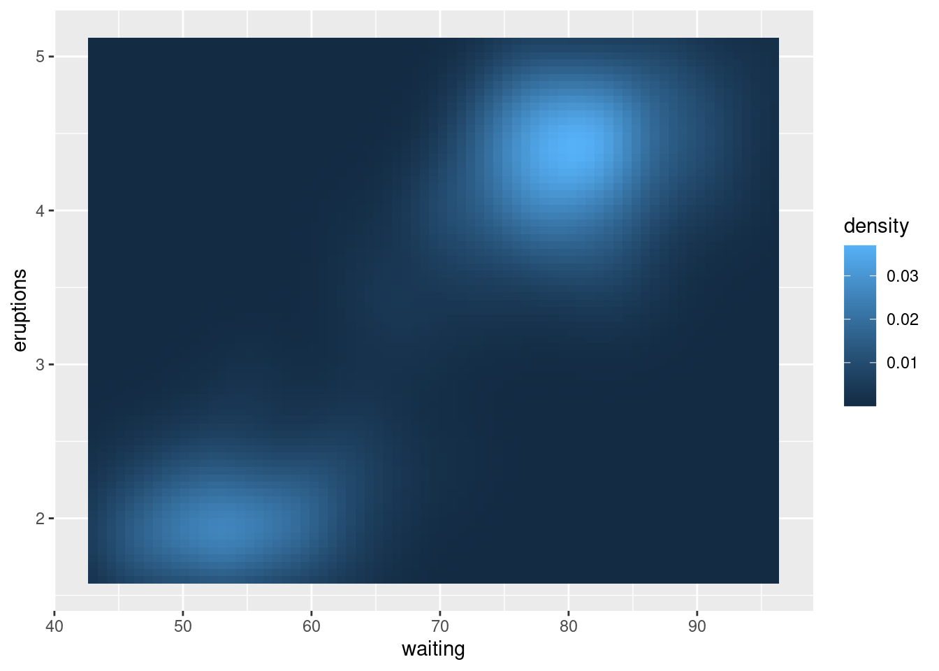
## Tile/Raster
::: {.grid}
::: {.g-col-6}
```{r}
#| filename: R
ggplot(faithfuld, aes(waiting, eruptions)) +
  geom_tile(aes(fill = density))
```
:::
::: {.g-col-6}
```{r}
#| filename: R
ojs_define(ojs_faithfuld = faithfuld)
```
```{ojs}
//| filename: OJS
faithfuld = transpose(ojs_faithfuld)
```
```{ojs}
//| filename: OJS
Plot.plot({
  marks: [
    Plot.raster(
      faithfuld,
      { x: "waiting", y: "eruptions", fill: "density", interpolate: "nearest" }
    )
  ]
})
```
:::
:::
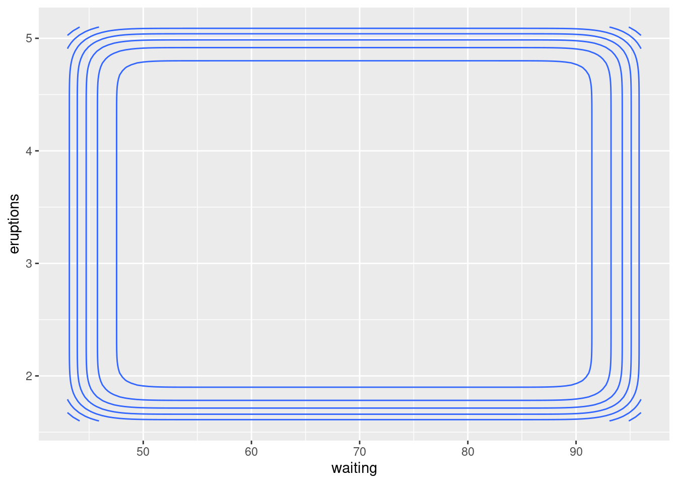
## 2D density
::: {.grid}
::: {.g-col-6}
```{r}
#| filename: R
ggplot(faithfuld, aes(waiting, eruptions)) +
  geom_density_2d()
```
:::
::: {.g-col-6}
```{ojs}
//| filename: OJS
Plot.plot({
  marks: [
    Plot.density(
      faithfuld,
      { x: "eruptions", y: "waiting"  }
    ),
    Plot.dot(
      faithfuld,
      { x: "eruptions", y: "waiting" }
    ),
  ],
  marginLeft: 50,
  marginBottom: 50
})
```
:::
:::
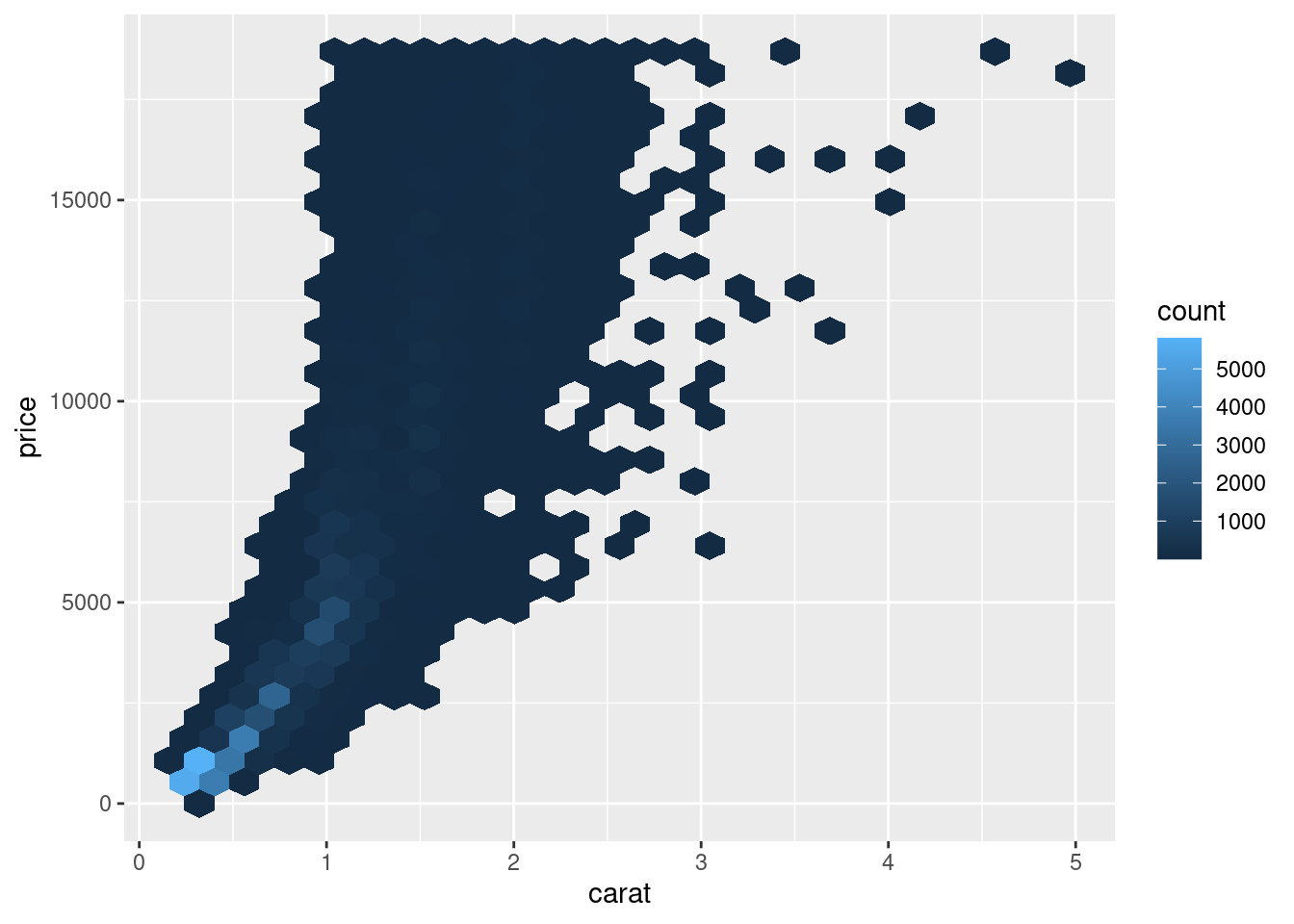
## Hex
::: {.grid}
::: {.g-col-6}
```{r}
#| filename: R
ggplot(diamonds, aes(carat, price)) +
  geom_hex()
```
:::
::: {.g-col-6}
```{r}
#| filename: R
ojs_define(ojs_diamonds = diamonds)
```
```{ojs}
//| filename: OJS
diamonds = transpose(ojs_diamonds)
```
```{ojs}
//| filename: OJS
Plot.plot({
  marks: [
    Plot.hexgrid(),
    Plot.dot(
      diamonds,
      Plot.hexbin(
        { r: "count" },
        { x: "carat", y: "price", fill: "currentColor" }
      )
    ),
  ],
  marginLeft: 50,
  marginBottom: 50
})
```
:::
:::
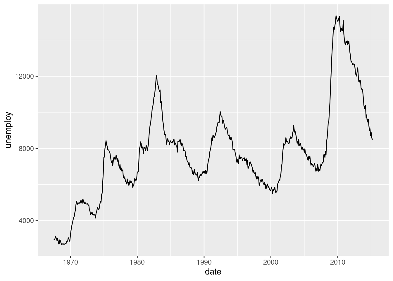
## Line
::: {.grid}
::: {.g-col-6}
```{r}
#| filename: R
ggplot(economics, aes(date, unemploy)) +
  geom_line()
```
:::
::: {.g-col-6}
```{r}
#| filename: R
ojs_define(ojs_economics = economics)
```
```{ojs}
//| filename: OJS
economics = transpose(ojs_economics)
```
```{ojs}
//| filename: OJS
Plot.plot({
  marks: [
    Plot.line(
      economics,
      { x: "date", y: "unemploy" }
    )
  ],
  grid: true
})
```
:::
:::
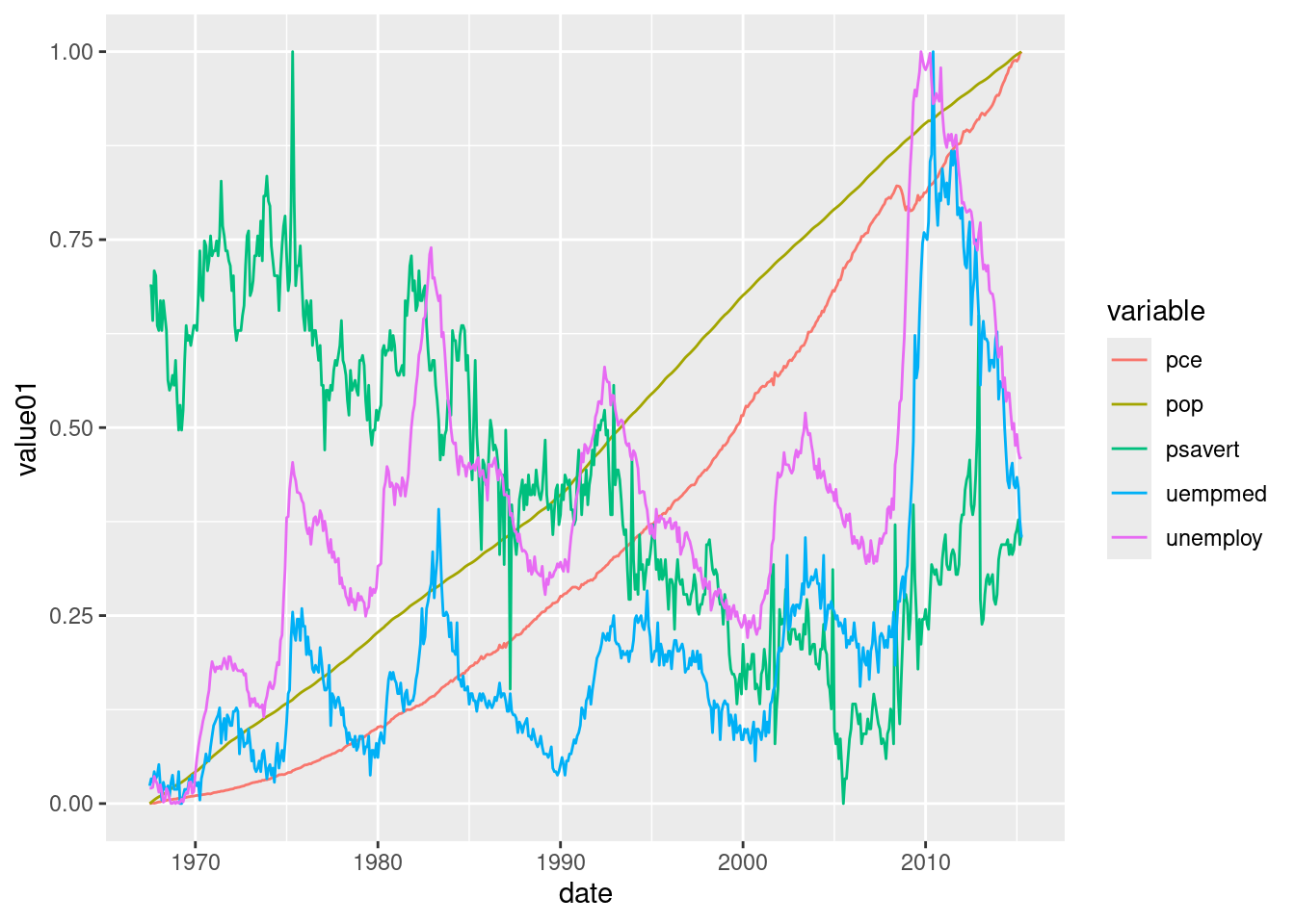
### With categorical colors
::: {.grid}
::: {.g-col-6}
```{r}
#| filename: R
ggplot(economics_long, aes(date, value01, colour = variable)) +
  geom_line()
```
:::
::: {.g-col-6}
```{ojs}
//| filename: OJS
Plot.plot({
  color: {
    legend: true
  },
  marks: [
    Plot.line(
      economics,
      { x: "date", y: "value01", stroke: "variable" }
    )
  ],
  grid: true
})
```
:::
:::
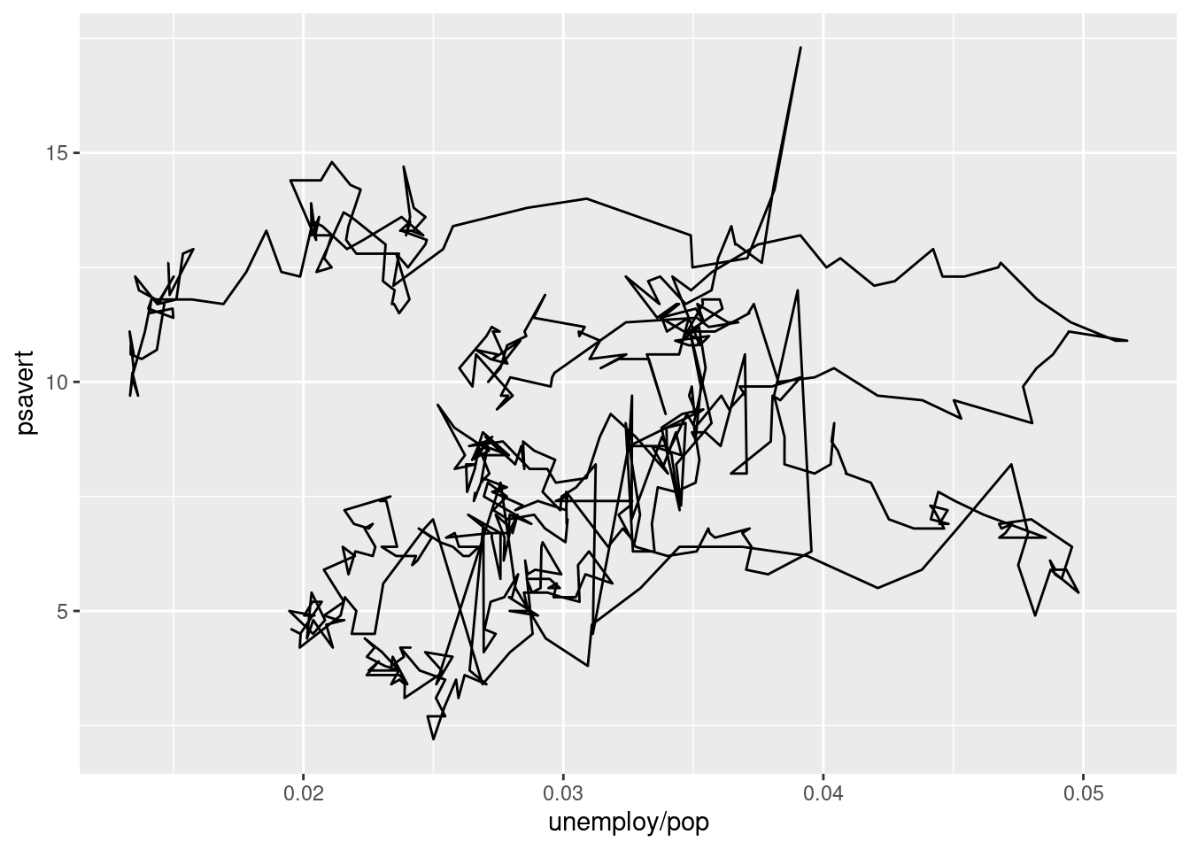
## Path
::: {.grid}
::: {.g-col-6}
```{r}
#| filename: R
ggplot(economics, aes(unemploy/pop, psavert)) +
  geom_path()
```
:::
::: {.g-col-6}
```{ojs}
//| filename: OJS
Plot.plot({
  marks: [
    Plot.line(economics, {
      x: (d) => d.unemploy / d.pop,
      y: "psavert",
      z: null,
      stroke: (d) => d.date
    })
  ],
  grid: true,
})
```
:::
:::