Sys.Date()[1] "2026-09-27"R code can be executed inline: `r Sys.Date()` renders as 2026-09-27.
R code can also be executed in code chunks.
```{r}
Sys.Date()
```
This shows the source code and output.
Sys.Date()[1] "2026-09-27"Here is another example with R source code and output.
data(iris)
head(iris[,1:2])| Sepal.Length | Sepal.Width |
|---|---|
| 5.1 | 3.5 |
| 4.9 | 3.0 |
| 4.7 | 3.2 |
| 4.6 | 3.1 |
| 5.0 | 3.6 |
| 5.4 | 3.9 |
Code chunk behavior is controlled with chunk options. In R chunks, each option starts with #| and uses YAML key: value syntax, for example, #| eval: false.
In this example, the R source code and results are hidden but the code is evaluated.
```{r}
#| eval: true
#| echo: false
#| results: hide
Sys.Date()
```
Source code blocks can be folded.
```{r}
#| code-fold: true
Sys.Date()
```Sys.Date()[1] "2026-09-27"Quarto does not provide built-in output folding, so this template uses the quarto-collapse-output extension.
```{r}
#| output-fold: true
Sys.Date()
```Sys.Date()[1] "2026-09-27"Use filename to display a filename above a code chunk.
```{r}
#| filename: R code
Sys.Date()
```
R code
Sys.Date()Enable line numbers using code-line-numbers: true.
```{r}
#| code-line-numbers: true
Sys.Date()
sessionInfo()
```An example showing Bash code generated from R:
```{r}
#| attr-output: "filename='bash'"
#| class-output: bash
#| echo: false
d <- "custom"
cat(paste("mkdir", d))
```
bash
mkdir customSee Quarto’s execution options and HTML code options.
For simple cases, tables can be manually created in Markdown.
|speed|dist|
|-----|----|
|4    |   2|
|4    |  10|
|7 | 4|| speed | dist |
|---|---|
| 4 | 2 |
| 4 | 10 |
| 7 | 4 |
A simple table using knitr::kable().
library(knitr)
kable(head(iris))| Sepal.Length | Sepal.Width | Petal.Length | Petal.Width | Species |
|---|---|---|---|---|
| 5.1 | 3.5 | 1.4 | 0.2 | setosa |
| 4.9 | 3.0 | 1.4 | 0.2 | setosa |
| 4.7 | 3.2 | 1.3 | 0.2 | setosa |
| 4.6 | 3.1 | 1.5 | 0.2 | setosa |
| 5.0 | 3.6 | 1.4 | 0.2 | setosa |
| 5.4 | 3.9 | 1.7 | 0.4 | setosa |
```{r}
#| column: body-outset
#| label: tbl-dual-table
#| tbl-cap: "Example"
#| tbl-subcap:
#|   - "Cars"
#|   - "Pressure"
#| layout-ncol: 2

kable(head(cars))
kable(head(pressure))
```| speed | dist |
|---|---|
| 4 | 2 |
| 4 | 10 |
| 7 | 4 |
| 7 | 22 |
| 8 | 16 |
| 9 | 10 |
| temperature | pressure |
|---|---|
| 0 | 0.0002 |
| 20 | 0.0012 |
| 40 | 0.0060 |
| 60 | 0.0300 |
| 80 | 0.0900 |
| 100 | 0.2700 |
Figures and tables can be numbered and cross-referenced by assigning a label that starts with fig- or tbl-, respectively. For example, @tbl-dual-table references the table above and renders as Table 1.
```{r}
#| tbl-cap: This table is in the margin.
#| column: margin

head(cars)
```| speed | dist |
|---|---|
| 4 | 2 |
| 4 | 10 |
| 7 | 4 |
| 7 | 22 |
| 8 | 16 |
| 9 | 10 |
An interactive table using rmarkdown::paged_table().
library(rmarkdown)
rmarkdown::paged_table(head(iris))| Sepal.Length | Sepal.Width | Petal.Length | Petal.Width | Species |
|---|---|---|---|---|
| 5.1 | 3.5 | 1.4 | 0.2 | setosa |
| 4.9 | 3.0 | 1.4 | 0.2 | setosa |
| 4.7 | 3.2 | 1.3 | 0.2 | setosa |
| 4.6 | 3.1 | 1.5 | 0.2 | setosa |
| 5.0 | 3.6 | 1.4 | 0.2 | setosa |
| 5.4 | 3.9 | 1.7 | 0.4 | setosa |
The gt package provides a grammar of tables with extensive customization options.
library(gt)

iris |>
    group_by(Species) |>
    slice(1:4) |>
    gt() |>
    cols_label(
      Sepal.Length = "Sepal Length", Sepal.Width = "Sepal Width",
      Petal.Length = "Petal Length", Petal.Width = "Petal Width"
    ) |>
    tab_source_note(
        source_note = md("Source: Iris data. Anderson, 1936; Fisher, 1936)")
)| Sepal Length | Sepal Width | Petal Length | Petal Width |
|---|---|---|---|
| setosa | |||
| 5.1 | 3.5 | 1.4 | 0.2 |
| 4.9 | 3.0 | 1.4 | 0.2 |
| 4.7 | 3.2 | 1.3 | 0.2 |
| 4.6 | 3.1 | 1.5 | 0.2 |
| versicolor | |||
| 7.0 | 3.2 | 4.7 | 1.4 |
| 6.4 | 3.2 | 4.5 | 1.5 |
| 6.9 | 3.1 | 4.9 | 1.5 |
| 5.5 | 2.3 | 4.0 | 1.3 |
| virginica | |||
| 6.3 | 3.3 | 6.0 | 2.5 |
| 5.8 | 2.7 | 5.1 | 1.9 |
| 7.1 | 3.0 | 5.9 | 2.1 |
| 6.3 | 2.9 | 5.6 | 1.8 |
| Source: Iris data. Anderson, 1936; Fisher, 1936) | |||
The htmlTable package creates styled HTML tables from R objects.
library(htmlTable)

iris1 <- iris[c(1:4,51:53,105:108),]
htmlTable(iris1, rgroup=unique(iris1$Species), n.rgroup=rle(as.character(iris1$Species))$lengths)| Sepal.Length | Sepal.Width | Petal.Length | Petal.Width | Species | |
|---|---|---|---|---|---|
| setosa | |||||
| 1 | 5.1 | 3.5 | 1.4 | 0.2 | setosa |
| 2 | 4.9 | 3 | 1.4 | 0.2 | setosa |
| 3 | 4.7 | 3.2 | 1.3 | 0.2 | setosa |
| 4 | 4.6 | 3.1 | 1.5 | 0.2 | setosa |
| versicolor | |||||
| 51 | 7 | 3.2 | 4.7 | 1.4 | versicolor |
| 52 | 6.4 | 3.2 | 4.5 | 1.5 | versicolor |
| 53 | 6.9 | 3.1 | 4.9 | 1.5 | versicolor |
| virginica | |||||
| 105 | 6.5 | 3 | 5.8 | 2.2 | virginica |
| 106 | 7.6 | 3 | 6.6 | 2.1 | virginica |
| 107 | 4.9 | 2.5 | 4.5 | 1.7 | virginica |
| 108 | 7.3 | 2.9 | 6.3 | 1.8 | virginica |
The kableExtra and formattable packages provide advanced table styling.
library(kableExtra)

iris[c(1:4,51:53,105:108),] |>
  mutate(Sepal.Length=color_bar("lightsteelblue")(Sepal.Length)) |>
  mutate(Sepal.Width=color_tile("white","orange")(Sepal.Width)) |>
  mutate(Species=cell_spec(Species,"html",color="white",bold=T,
    background=c("#8dd3c7","#fb8072","#bebada")[factor(Species)])) |>
  kable("html",escape=F) |>
  kable_styling(bootstrap_options=c("striped","hover","responsive"),
                full_width=F,position="left") |>
column_spec(5,width="3cm")| Sepal.Length | Sepal.Width | Petal.Length | Petal.Width | Species | |
|---|---|---|---|---|---|
| 1 | 5.1 | 3.5 | 1.4 | 0.2 | setosa |
| 2 | 4.9 | 3.0 | 1.4 | 0.2 | setosa |
| 3 | 4.7 | 3.2 | 1.3 | 0.2 | setosa |
| 4 | 4.6 | 3.1 | 1.5 | 0.2 | setosa |
| 51 | 7.0 | 3.2 | 4.7 | 1.4 | versicolor |
| 52 | 6.4 | 3.2 | 4.5 | 1.5 | versicolor |
| 53 | 6.9 | 3.1 | 4.9 | 1.5 | versicolor |
| 105 | 6.5 | 3.0 | 5.8 | 2.2 | virginica |
| 106 | 7.6 | 3.0 | 6.6 | 2.1 | virginica |
| 107 | 4.9 | 2.5 | 4.5 | 1.7 | virginica |
| 108 | 7.3 | 2.9 | 6.3 | 1.8 | virginica |
The DT package creates interactive data tables.
library(DT)

iris |>
  slice(1:15) |>
datatable(options = list(pageLength = 7))The reactable package creates advanced interactive tables.
library(reactable)

reactable(iris[sample(1:150,10),],
  columns = list(
    Sepal.Length = colDef(name = "Sepal Length"),
    Sepal.Width = colDef(name = "Sepal Width"),
    Petal.Length = colDef(name = "Petal Length"),
    Petal.Width = colDef(name = "Petal Width")
  ),
  striped = TRUE,
  highlight = TRUE,
  filterable = TRUE
)
The reactablefmtr package can simplify and extend reactable tables.
Use the out-width chunk option to control an image’s displayed width.
The image below is displayed at 300 pixels wide.
```{r}
#| out-width: 300px
knitr::include_graphics("assets/image.webp")
```
The image below is displayed at 75 pixels wide and has a caption.
```{r}
#| out-width: 75px
#| fig-cap: This is a caption
knitr::include_graphics("assets/image.webp")
```
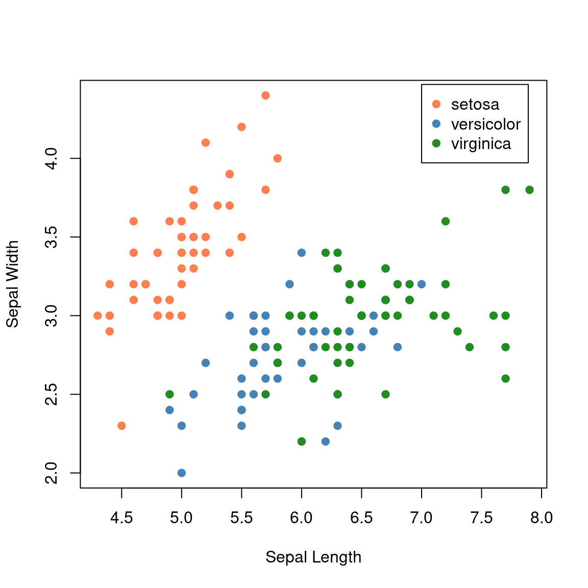
See Quarto’s figure documentation for more information. R-generated plots are demonstrated below.
{
  plot(x=iris$Sepal.Length,y=iris$Sepal.Width,
      col=c("coral","steelblue","forestgreen")[iris$Species],
      xlab="Sepal Length",ylab="Sepal Width",pch=19)

  legend(x=7,y=4.47,legend=c("setosa","versicolor","virginica"),
        col=c("coral","steelblue","forestgreen"),pch=19)
}
```{r}
#| column: screen-inset-shaded
#| layout-nrow: 1
#| fig-cap:
#|   - "Scatterplot of speed vs distance"
#|   - "Pairwise scatterplot of all variables"
#|   - "Scatterplot of temperature vs pressure"

plot(cars)
plot(iris)
plot(pressure)
```


```{r}
#| column: margin

plot(cars)
```
The ggplot2 package provides a grammar of graphics for creating static plots.
library(ggplot2)

iris |>
  ggplot(aes(x=Sepal.Length,y=Sepal.Width,col=Species))+
  geom_point(size=2)+
  labs(x="Sepal Length",y="Sepal Width")+
  theme_report()
The highcharter package provides an R interface to the Highcharts JavaScript library.
library(highcharter)

h <- hchart(iris,"scatter",hcaes(x="Sepal.Length",y="Sepal.Width",group="Species")) |>
  hc_xAxis(title=list(text="Sepal Length"),crosshair=TRUE) |>
  hc_yAxis(title=list(text="Sepal Width"),crosshair=TRUE) |>
  hc_chart(zoomType="xy",inverted=FALSE) |>
  hc_legend(verticalAlign="top",align="right") |>
  hc_size(height=400)

htmltools::tagList(list(h))The plotly package provides an R interface to the Plotly.js JavaScript library.
library(plotly)

p <- iris |>
  plot_ly(x=~Sepal.Length,y=~Sepal.Width,color=~Species,width=500,height=400) |>
  add_markers()
pplotly::ggplotly() converts a ggplot2 plot into an interactive Plotly graphic.
library(plotly)

p <- iris |>
  ggplot(aes(x=Sepal.Length,y=Sepal.Width,col=Species))+
  geom_point()+
  labs(x="Sepal Length",y="Sepal Width")+
  theme_bw(base_size=12)

ggplotly(p,width=500,height=400)The ggiraph package adds tooltips, hover effects, and other interactions to ggplot2 graphics.
library(ggiraph)

p <- ggplot(iris,aes(x=Sepal.Length,y=Petal.Length,colour=Species))+
      geom_point_interactive(aes(tooltip=paste0("<b>Petal Length:</b> ",Petal.Length,"\n<b>Sepal Length: </b>",Sepal.Length,"\n<b>Species: </b>",Species)),size=2)+
  theme_bw()

tooltip_css <- "background-color:#e7eef3;font-family:Roboto;padding:10px;border-style:solid;border-width:2px;border-color:#125687;border-radius:5px;"

girafe(code=print(p),
  options=list(
    opts_hover(css="cursor:pointer;stroke:black;fill-opacity:0.3"),
    opts_zoom(max=5),
    opts_tooltip(css=tooltip_css,opacity=0.9)
  )
)The dygraphs package provides R bindings to the dygraphs JavaScript library for interactive time-series charts.
library(dygraphs)

lungDeaths <- cbind(ldeaths, mdeaths, fdeaths)
dygraph(lungDeaths,main="Deaths from Lung Disease (UK)") |>
dyOptions(colors=c("#66C2A5","#FC8D62","#8DA0CB"))The networkD3 package creates interactive network graphs using D3.js.
library(networkD3)

data(MisLinks,MisNodes)
forceNetwork(Links=MisLinks,Nodes=MisNodes,Source="source",
             Target="target",Value="value",NodeID="name",
Group="group",opacity=0.4)The leaflet package provides R bindings to the Leaflet JavaScript library.
library(leaflet)

leaflet(height=500,width=700) |>
  addTiles(urlTemplate='https://{s}.tile.openstreetmap.org/{z}/{x}/{y}.png') |>
  #addProviderTiles(providers$Esri.NatGeoWorldMap) |>
  addMarkers(lat=57.639327,lng=18.288534,popup="RaukR") |>
setView(lat=57.639327,lng=18.288534,zoom=15)The crosstalk package links selections and filters across compatible HTML widgets that share a SharedData object.
library(crosstalk)

shared_quakes <- SharedData$new(quakes[sample(nrow(quakes), 100),])
lf <- leaflet(shared_quakes,height=300) |>
        addTiles(urlTemplate='https://{s}.tile.openstreetmap.org/{z}/{x}/{y}.png') |>
        addMarkers()
py <- plot_ly(shared_quakes,x=~depth,y=~mag,size=~stations,height=300) |>
        add_markers()

htmltools::div(lf,py)Quarto supports Observable JS for interactive visualizations in the browser.
Pass data from R to OJS:
irism <- iris
colnames(irism) <- gsub("[.]","_",tolower(colnames(irism)))
ojs_define(ojsd = irism)
ojsdata = transpose(ojsd)Display the data as a table:
viewof filtered_table = Inputs.table(ojsdata)Define inputs:
viewof x = Inputs.select(Object.keys(ojsdata[0]), {value: "sepal_length", multiple: false, label: "X axis"})viewof y = Inputs.select(Object.keys(ojsdata[0]), {value: "sepal_width", multiple: false, label: "Y axis"})Display the plot:
Plot.plot({
  marks: [
    Plot.dot(ojsdata, {
      x: x,
      y: y,
      fill: "species",
      title: (d) =>
        `${d.species} \n Petal length: ${d.petal_length} \n Sepal length: ${d.sepal_length}`
    })
  ],
  grid: true
})
See Quarto’s Observable JS documentation.
Icons can be generated from R with the fontawesome package.
`r fontawesome::fa('lightbulb')`
height and fill are optional arguments.
`r fontawesome::fa('lightbulb',height='30px',fill='steelblue')`
See Font Awesome for a full list of icons.
R version 4.6.1 (2026-06-24)
Platform: x86_64-pc-linux-gnu
Running under: Ubuntu 24.04.5 LTS

Matrix products: default
BLAS:   /usr/lib/x86_64-linux-gnu/openblas-pthread/libblas.so.3
LAPACK: /usr/lib/x86_64-linux-gnu/openblas-pthread/libopenblasp-r0.3.26.so;  LAPACK version 3.12.0

locale:
 [1] LC_CTYPE=C.UTF-8       LC_NUMERIC=C           LC_TIME=C.UTF-8
 [4] LC_COLLATE=C.UTF-8     LC_MONETARY=C.UTF-8    LC_MESSAGES=C.UTF-8
 [7] LC_PAPER=C.UTF-8       LC_NAME=C              LC_ADDRESS=C
[10] LC_TELEPHONE=C         LC_MEASUREMENT=C.UTF-8 LC_IDENTIFICATION=C

time zone: UTC
tzcode source: system (glibc)

attached base packages:
[1] stats     graphics  grDevices utils     datasets  methods   base

other attached packages:
 [1] rmarkdown_2.32    fontawesome_0.5.3 crosstalk_1.2.2   leaflet_2.2.3
 [5] networkD3_0.4.1   dygraphs_1.1.1.6  ggiraph_0.9.6     plotly_4.12.1
 [9] highcharter_0.9.5 ggplot2_4.0.3     reactable_0.4.5   DT_0.34.0
[13] gt_1.3.0          formattable_0.2.1 kableExtra_1.4.1  htmlTable_2.5.0
[17] knitr_1.52        stringr_1.6.0     tidyr_1.3.2       dplyr_1.2.1

loaded via a namespace (and not attached):
 [1] tidyselect_1.2.1        viridisLite_0.4.3       farver_2.1.2
 [4] S7_0.2.2                fastmap_1.2.0           fontquiver_0.2.1
 [7] digest_0.6.39           timechange_0.4.0        lifecycle_1.0.5
[10] magrittr_2.0.5          compiler_4.6.1          rlang_1.3.0
[13] sass_0.4.10             tools_4.6.1             igraph_2.3.3
[16] yaml_2.3.12             data.table_1.18.6.1     labeling_0.4.3
[19] htmlwidgets_1.6.4       curl_8.0.0              xml2_1.6.0
[22] TTR_0.24.4              RColorBrewer_1.1-3      withr_3.0.3
[25] purrr_1.2.2             grid_4.6.1              gdtools_0.5.1
[28] xts_0.14.3              data.tree_1.2.0         scales_1.4.0
[31] MASS_7.3-65             cli_3.6.6               generics_0.1.4
[34] otel_0.2.0              rlist_0.4.6.2           rstudioapi_0.19.0
[37] httr_1.4.9              commonmark_2.0.0        cachem_1.1.0
[40] assertthat_0.2.1        base64enc_0.1-6         vctrs_0.7.3
[43] jsonlite_2.0.0          fontBitstreamVera_0.1.1 litedown_0.11
[46] systemfonts_1.3.2       jquerylib_0.1.4         quantmod_0.4.29
[49] glue_1.8.1              reactR_0.6.1            lubridate_1.9.5
[52] stringi_1.8.9           gtable_0.3.6            tibble_3.3.1
[55] pillar_1.11.1           htmltools_0.5.9         R6_2.6.1
[58] textshaping_1.0.5       evaluate_1.0.5          lattice_0.22-9
[61] markdown_2.0            backports_1.5.1         broom_1.0.13
[64] bslib_0.12.0            fontLiberation_0.1.0    Rcpp_1.1.2
[67] svglite_2.2.2           checkmate_2.3.4         xfun_0.61
[70] fs_2.1.0                zoo_1.9-1               pkgconfig_2.0.3